Prev

The KMV Sketch, Update V(k^th) Rule

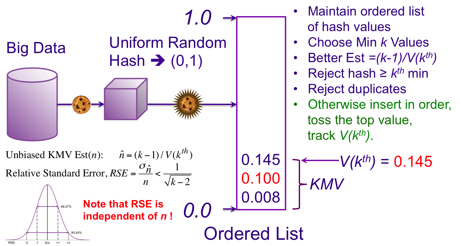
Our final rules:

If the cache is presented with a hash value that is less than V(k^th) and not a duplicate, we insert the new value in order, remove what was the V(k^th) value and replace it with whatever was next in order, which becomes the new V(k^th) value.

If the cache has been presented with less than k values, the estimate equals the current count of values in the cache. This is also known as Exact Mode (as opposed to Estimation Mode).

We now have a complete KMV sketch, with some amazing properties:

• The sketch has a fixed upper bound size of k values.
• De-duplication is part of the algorithm.
• If the sketch has retained less than k values, the resulting estimate is exact and is just the count of the values in the cache. Otherwise, the unbiased estimate of the unique values seen by the sketch is (k-1)/V(k^th)[1].
• The Relative Standard Error or RSE of the estimate, for this simple KMV Sketch, is ≤ 1/sqrt(k-2)[1], which is a constant and independent of n, the number of uniques presented to the sketch (See Accuracy). For large enough values of k the error distribution is roughly Gaussian, which makes preditions of confidence intervals relatively straightforward.

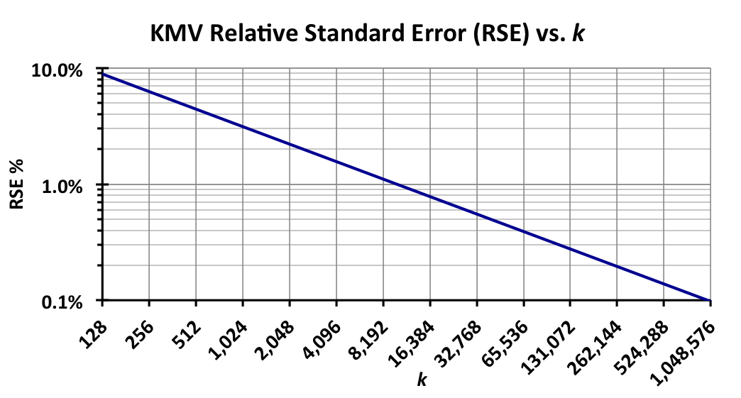
To figure out what value of k is required, you must first determine what level of accuracy is required for your application. The graph below can serve as a guide.

The RSE corresponds to +/- one Standard Deviation of the Gaussian distribution, which is equivalent to a confidence of 68%. To obtain the Relative Error (RE, no longer “Standard”) at 95% confidence and the same value of k you multiply the RSE value by two. For example, reading from the chart, choosing k = 4096 corresponds to an RSE of +/- 1.6% with 68% confidence. That same size sketch will have a Relative Error of +/- 3.2% with 95% confidence.

The values of k are shown as powers of 2 for a reason. From an implementation point-of-view, choosing internal cache sizes that are powers of 2 improves performance and is simpler to implement.

Note that the sketch algorithms implemented in the DataSketches library are more sophisticated than the simple KMV sketch outlined here and the corresponding estimation equations are slightly different and the error bounds equations are much more complex. Don’t worry, all the complexity is handled for you in the library. This will be discussed more extensively in other sections.

[1] For those interested in the mathematical proofs, Giroire has a straightforward and easy-to-follow development.

Prev