Suppose you have a new Internet company that sells Mobile Apps and Music. Your internal reporting system collects log data from two main sources: your web servers and your Financial Transactions System that records purchases and handles credit cards and authentication. The data logs from these two systems might look something like this:
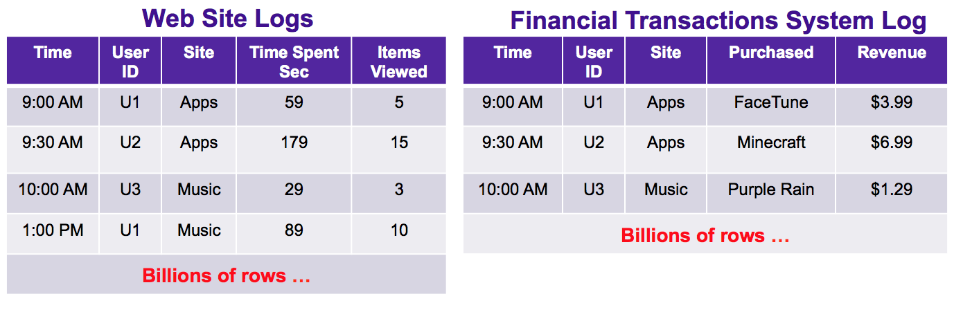
The web server logs contain information such as a time-stamp, a user identifier (obfuscated, of course), the site visited, a time-spent metric, and a number of items viewed metric. The financial logs contain information such as a time-stamp, a user identifier, the site visited, the purchased item and revenue received for the item.
From these two simple sets of data there are many queries that we would like to make, and among those, some very natural queries might include the following:
This all sounds pretty “ho-hum”. However, and fortunately for you, your company has become wildly successful and both the web logs and financial transactions log consist of billions of records per day.
If you have any experience with answering these types of queries with massive data sets it should give you pause. And, if you are already attempting to answer similar queries with your massive data, you might wonder why answering these queries requires so many resources and takes hours, or sometimes days to compute.
Computer Scientists have known about these types of queries for a long time, but not much attention was paid to the impact of these queries until the Internet exploded and Big Data reared its ugly head.
It has been proved (and can be intuited, with some thought) that in order to compute these queries exactly, assuming nothing about the input stream and, for the quantiles case, without any restrictions on the number of quantiles requested, requires the query process to keep copies of every unique value encountered.
This is staggering. In order to count the exact number of unique visitors to a web site that has a billion users per day, requires the query process to keep on hand a billion records of all the unique visitors it has ever seen. Unique identifier counts are not additive either, so no amount of parallelism will help you. You cannot add the number of identifiers from the apps data site to the number of identifiers from the music site because of identifiers that appear on both sites, i.e., the duplicates.
The exact quantiles query is even worse. Not only does it need to keep a copy of every item seen, it needs to sort them to boot!
Here is a very fundamental business question: “Do you really need 10+ digits of accuracy in the answers to your queries? This leads to the fundamental premise of this entire branch of Computer Science:
If an approximate answer is acceptable, then it is possible that there are algorithms that allow you to answer these queries orders-of-magnitude faster.
This, of course, assumes that you care about query responsiveness and speed; that you care about resource utilization; and if you need to accept some approximation, that you care about knowing something about the accuracy that you end up with.
Sketches, the informal name for these algorithms, offer an excellent solution to these types of queries, and in some cases may be the only solution.
Instead of requiring to keep such enormous data on-hand, sketches have small data structures that are usually kilobytes in size, orders-of-magnitude smaller than required by the exact solutions. Sketches are also streaming algorithms, in that they only need to see each incoming item once.

The first big win is the size of the query process on the right has been reduced many orders-of-magnitude. Unfortunately, the process is still slow (although it was faster than before), because the single query process must sequentially scan through all the raw data on the left, which is huge.
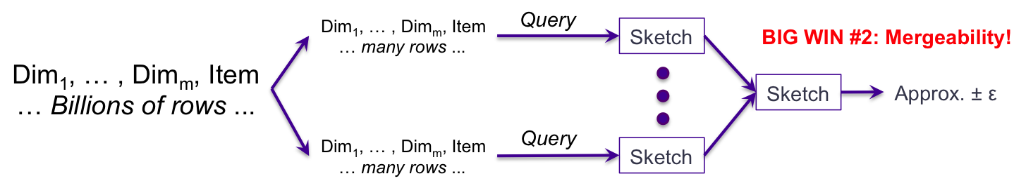
The second big win is that the sketch data structures are “Mergeable”, which enables parallel processing. The input data can be partitioned into many fragments. At query time each partition is processed with its own sketch. Once all the sketches have completed their scan of their associated data, the merging (or unioning) of the sketches is very fast. This provides another speed performance boost. But there is a catch. Typical user data is highly skewed and is unlikely to be evenly divided across the partitions. The overall speed of the processing is now determined by the most heavily loaded partition.
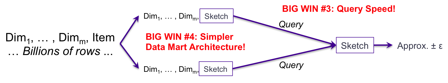
The placement of the query in this diagram illustrates Big Win #3. The primary difference between this diagram and the previous one is where in the data flow the query is performed and how much work the query process has to do. The Big Win #2 is an improvement over #1, but still requires the query process to process raw data in partitions, which still can be huge.
However, if we do the sketching of each of the partitions at the same time we do the partitioning we create an intermediate “hyper-cube” or “data-mart” architecture where each row becomes a summary row for that partition. The intermediate staging no longer has any raw data. It only consists of a single row for each dimension combination. And the metric columns for that row contain the aggregation of whatever other additive metrics you require, plus a column that contains the binary image of a sketch. At query time, the only thing the query process needs to do is select the appropriate rows needed for the query and merge the sketches from those rows. We have measured the merge speed of the Theta sketches in the range of 10 to 20 million sketches per second in a large system with real data. This is the Big Win #3.
Placing the sketch, along with other metrics into a data-mart architecture vastly simplifies the design of the system, which is the Big Win #4.
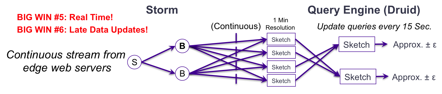
Processing the continuous real-time stream from the edge web servers is possible with Storm that splits the stream into multiple parallel streams based on the dimensions. These can be ingested into Druid in real-time and sent directly to sketches organized by time and dimension combination. In our Flurry system the time resolution is 1 minute. The reporting web servers query these 1 minute sketches on 15 second intervals. This Real-time, Big Win #5, is simply not feasible without sketches. In addition, these sketches can be correctly updated with late data, which happens frequently with mobile traffic. This becomes the Big Win #6.
It has been our experience at Yahoo/VM, that a good implementation of these large analysis systems using sketches reduces the overall cost of the system considerably. It is difficult to quote exact numbers as your mileage will vary as it is system and data dependent.
1The term “big data” is a popular term for truly massive data, and is somewhat ambiguous. For our usage here, it implies data (either in streams or stored) that is so massive that traditional analysis methods do not scale.
2count distinct is the formal term, borrowed from SQL that has an operator by that name, for the counting of just the distinct (or unique) items of a set ignoring all duplicates. For our usage here, it is reads more smoothly to just refer to distinct count or unique count.

