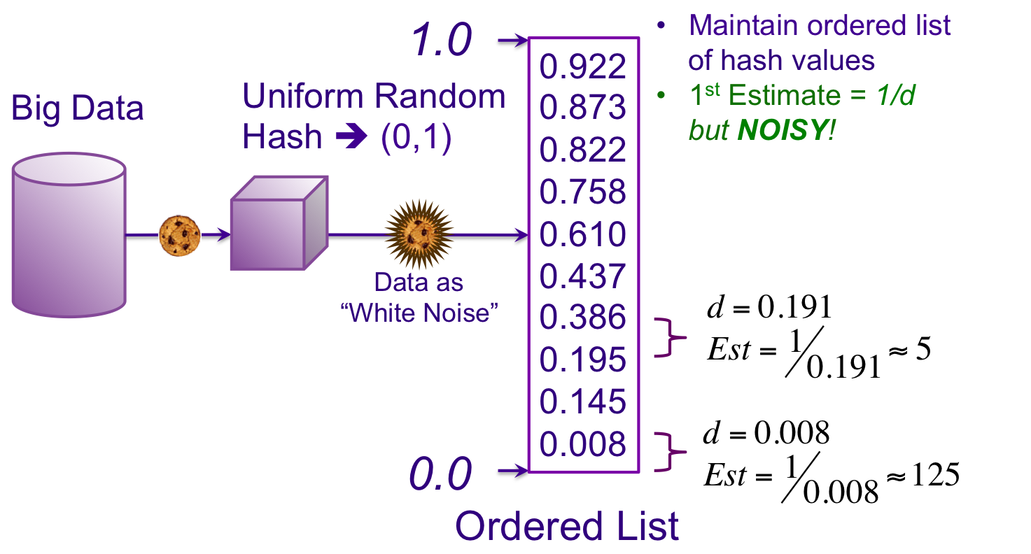
For this step we are going to cheat a little so that we can learn about estimation. We are going to cheat in that we are going to predetermine that our data source only has n = 10 unique values (so we don’t really need a sketch to estimate what we already know). We have loaded all 10 values into our ordered list. As one can see, the values are roughly evenly distributed between zero and one so our hash transform is doing its job.
How many hash values do we have to retain to compute the estimate of n, n̂, accurately? As you might expect, the more samples we retain, the more accurate will be our estimate.
Suppose we kept only one value, so k = 1, and we chose the smallest hash value out of all the hash values in the set, which, in this case, is 0.008. We could assume that since the hash values are random-uniform distributed that the separation between the hash values are roughly the same. Let’s label that separation between values as d. Our first estimator could be just dividing 1.0 by d. Unfortunately, 1/0.008 is about 125, which is way larger than 10. And as one can see, there is a lot of variation in the separation of each of the hash values. If the hash values had been ordered differently, the smallest hash value could have been the separation between the 3rd and 4th values. In this case our first estimator, 1/0.191 would be about 5, which is too small.

Clearly, our first estimator, 1/d, with a sample size of one is too noisy to be useful. However, what we do have is a simple formula for an estimate:
