This code example illustrates the use of 4 important bounds functions provided by the KLL sketches:
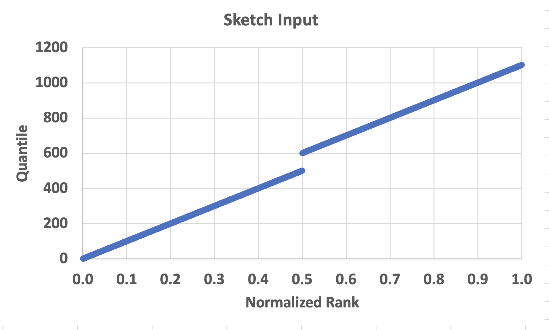
The input into the sketch is a simple monotonic sequence but with a big discontinuity in the middle. Then we extract the upper and lower bounds of both the rank and quantile domains on both sides of the discontinuity.
import org.testng.annotations.Test;

public class QuantileBoundsTest {
  private int n = 1000;
  private int k = 400;

  @Test
  public void exampleQuantileBounds( ) {
    KllDoublesSketch sk = KllDoublesSketch.newHeapInstance(k);
    for (int i = 1; i <= n; i++) {
      int j = (i > 500)? i + 100 : i; //note big jump at 501!
      sk.update(j);
    }

    double rankError = sk.getNormalizedRankError(false);
    println("Normalized Rank Error: +/- " + rankError);
    println("Absolute Rank Error  : +/- " + rankError * n);
    println("");

    double q1 = 500;
    println("q1: " + q1);
    double q2 = 620;
    println("q2: " + q2);

    double r1 = sk.getRank(q1);
    println("r1: " + r1);
    double r2 = sk.getRank(q2);
    println("r2: " + r2);
    println("");

    println("r1LB(r1): " + sk.getRankLowerBound(r1));
    println("r1UB(r1): " + sk.getRankUpperBound(r1));
    println("r2LB(r2): " + sk.getRankLowerBound(r2));
    println("r2UB(r2): " + sk.getRankUpperBound(r2));
    println("");

    println("q1LB(r1): " + sk.getQuantileLowerBound(r1));
    println("q1UB(r1): " + sk.getQuantileUpperBound(r1));
    println("q2LB(r2): " + sk.getQuantileLowerBound(r2));
    println("q2UB(r2): " + sk.getQuantileUpperBound(r2));
    println("");
  }

  private static void println(Object o) { System.out.println(o.toString()); }
}
Normalized Rank Error: +/- 0.0067762427270138155
Absolute Rank Error  : +/- 6.776242727013815

q1: 500.0
q2: 620.0
r1: 0.5
r2: 0.52

r1LB(r1): 0.4932237572729862
r1UB(r1): 0.5067762427270138
r2LB(r2): 0.5132237572729862
r2UB(r2): 0.5267762427270138

q1LB(r1): 494.0
q1UB(r1): 608.0
q2LB(r2): 614.0
q2UB(r2): 628.0

PASSED: exampleQuantileBounds
The sketch is configured with a k=400, which results in a normalized rank error of +/- .68%. Multiplying that by n produces the absolute (or natural) rank error of 6.8 relative to n of 1000.
The input stream of 1000 values has a big discontinuity starting at i = 501. So the actual sequence of inputs is 1 to 500 and 601 to 1100.

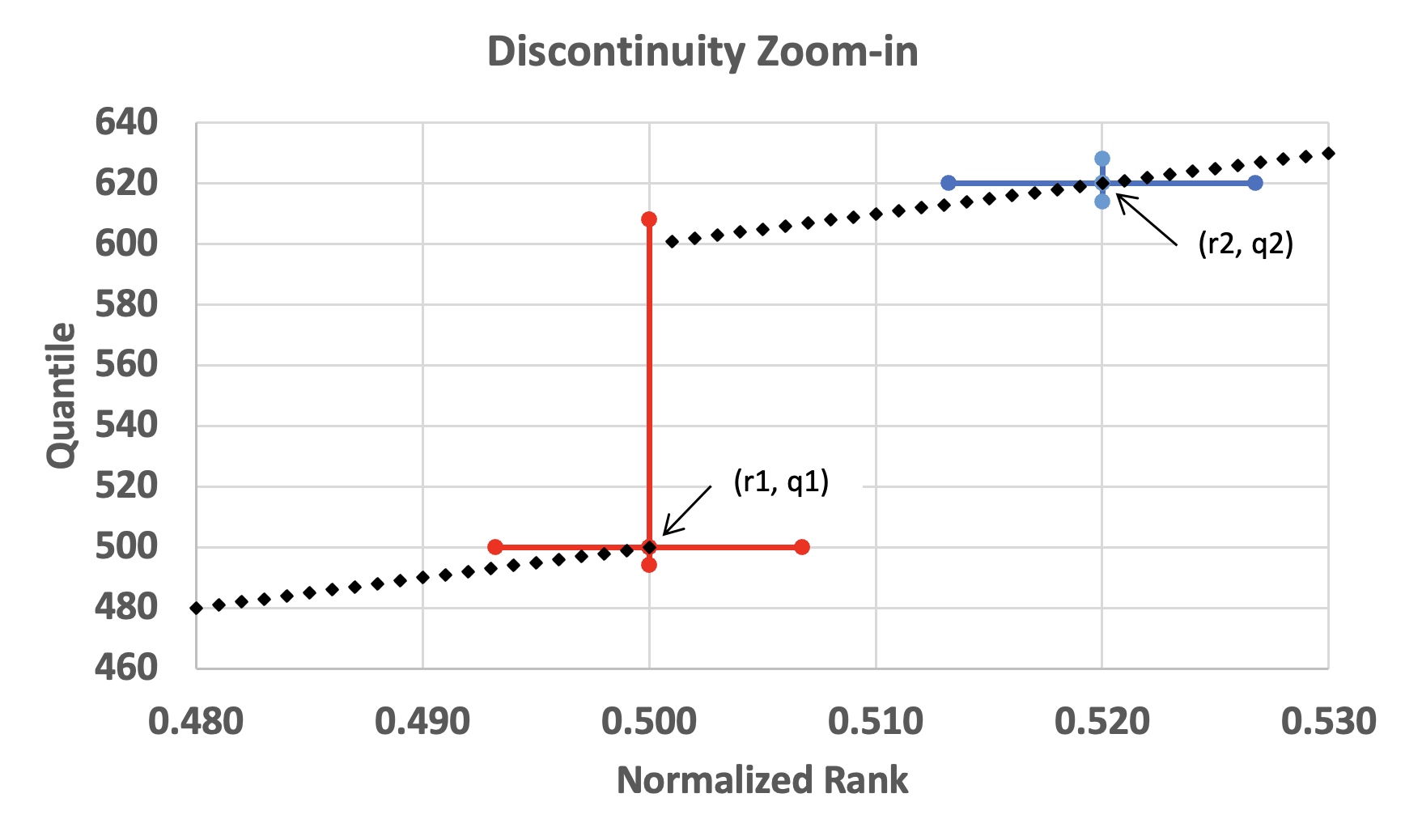
We choose two quantiles on either side of the discontinuity, 500 and 620, and get their respective ranks of 0.5 and 0.52. Note that because of the discontinuity the difference in the input quantiles is 120/1100 or ~10.9%, while the difference in their respective ranks is only 2%.
Next we compute the rank upper bound (UB) and rank lower bound (LB) of the two resulting ranks of 0.5 and 0.52, which are given above. Note that the UB - LB of each rank is about .013 which is 2 X .0067. This means that the true rank of each quantile is within the UB - LB range of ranks with a confidence of 99%, which is about +/- 2.6 standard deviations from the estimate.
Then we compute the quantile UB and LB of the same two resulting ranks of 0.5 and 0.52. Note that the UB - LB quantile range of r1 is 114/1100 or 10.4%, because in between the rank UB and LB is the discontinuity. These points are shown in the next plot

This graphically illustrates why the mathematical guarantee of error applies only to the rank domain, because the input quantile domian could have huge discontinuities. Nonetheless, we can say that the true quantile does lie within that UB - LB quantile range with a confidence of 99%. But we cannot guarantee anything about the UB - LB quantile difference and relate that to a quantile accuracy compared to the total range of the input values.
Our Classic, KLL, and REQ quantiles sketches are input insensitive and do not know or care what the input distribution looks like. It does not have to be a smooth and well behaved function. This is not the case with other heuristic quantile algorithms,