This is a real-time, key-value HLL mapping sketch that tracks approximate unique counts of identifiers (the values) associated with each key. An example might be tracking the number of unique user identifiers associated with each IP address. This map has been specifically designed for the use-case where the number of keys is quite large (many millions) and the distribution of identifiers per key is very skewed. A typical distribution where this works well is a power-law distribution of identifiers per key of the form y = Cx-α, where α < 0.5, and C is roughly ymax. For example, with 100M keys, over 75% of the keys would have only one identifier, 99% of the keys would have less than 20 identifiers, 99.9% would have less than 200 identifiers, and a very tiny fraction might have identifiers in the thousands.
This sketch is quite different from other sketches in the library:
Because all keys that have been seen by the sketch are retained, this sketch can grow to be quite large. The space consumed by this map is quite sensitive to the actual distribution of identifiers per key, so you should characterize and or experiment with your typical input streams. Nonetheless, our experiments on live streams of about 100M keys required space less than 1.4GB.
Given such highly-skewed distributions, using this map is far more efficient space-wise than the alternative of dedicating the library HllSketch per key. Based on our use cases, after subtracting the space required for key storage, the average bytes per key required for unique count estimation (see method getAverageSketchMemoryPerKey()) is about 10 bytes.
Assuming that the frequency distribution of your identifiers per key is roughly power-law with a log-log slope of about -1, the total storage required for this sketch can be roughly computed as
Size = (K + S) * T
    where K = Key size in bytes
          S = Average HLL Sketch Memory Per Key
          T = Total number of keys seen by the sketch
In our use-case we had a strong power-law distribution of IDs/key where the average HLL sketch memory per key was about 10. With 100M keys, the space consumed was about 1.4 GB. Nonetheless, the sketch tracks the memory usage for you and it can be obtained at any time with the getMemoryUsageBytes() method. The sketch also offers a getAverageSketchMemoryPerKey(), which estimates the value S in the above equation.
Internally, this map is implemented as a hierarchy of internal hash maps with progressively increasing storage allocated for unique count estimation. As a key acquires more identifiers it is “promoted” up to a higher internal map. The final map of keys is a map of compact HLL sketches.
The unique values in all the internal maps, except the final HLL map, are stored in a special form called a coupon. A coupon is a 16-bit value that fully describes a k=1024 HLL bin. It contains 10 bits of address and a 6-bit HLL value.
All internal maps use a prime number size and Knuth’s Open Addressing Double Hash (OADH) search algorithm.
The internal base map holds all the keys and each key is associated with one 16-bit value. Initially, the value is a single coupon. Once the key is promoted, this 16-bit field contains a reference to the internal map where the key is still active.
The intermediate maps between the base map and the final HLL map are of two types. The first few of these are called traverse maps where the coupons are stored as unsorted arrays. After the traverse maps are the coupon hash maps, where the coupons are stored in small OASH (Open Address Single Hash) hash tables.
All the intermediate maps support deletes and can dynamically grow and shrink as required by the input stream.
The sketch estimator algorithms are unbiased with a Relative Standard Error (RSE) of about 2.6% with 68% confidence, or equivalently, about 5.2% with a 95% confidence.
At the time this sketch was designed there was no requirement for merging these sketches, so the merge operation was never implemented. This sketch was designed to operate on a single server for real-time tracking and monitoring.
The accuracy behavior of the UniqueCountMap sketch will be similar to the following graph:
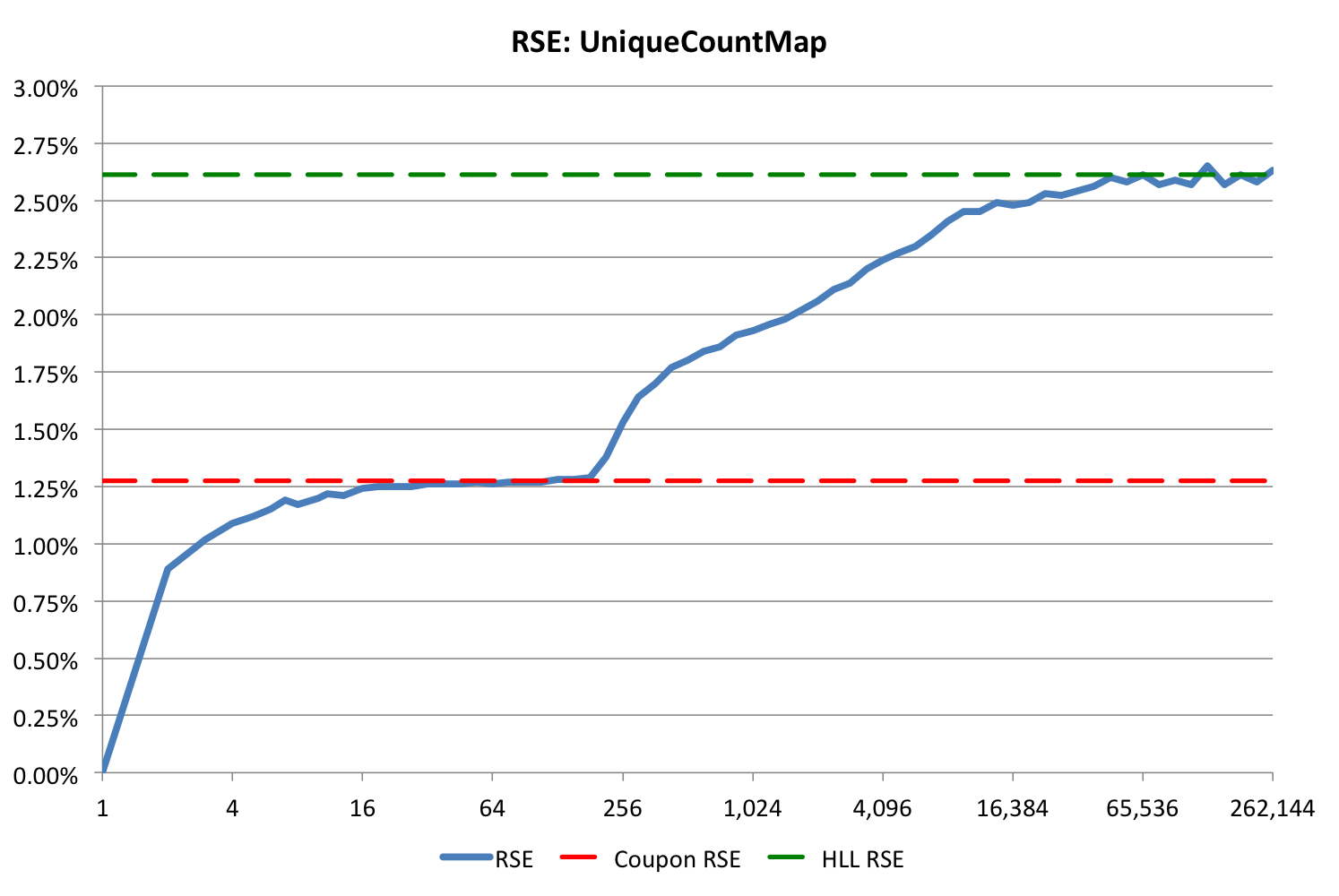
The blue curve is the RSE for the sketch and has two regions corresponding to two different estimator algorithms. The first estimator is for the low count region less than 192 uniques, and the second estimator is used for counts greater than 192.
The theoretical bound for the first estimator is shown as the red dashed line. The theoretical bound for the high range estimator is shown as the green dashed line.
The update/estimate speed behavior of the this sketch is dependent on the actual distribution of identifiers per key, so it is difficult to characterize. However, in our own testing with real data, we observed update/estimate speeds of less than 500 nanoseconds.

