These sketches provide the following capabilities:
Estimate the frequency of an item.
Return upper and lower bounds of any item, such that the true frequency is always between the upper and lower bounds.
Return a global maximum error that holds for all items in the stream.
Return an array of frequent items that qualify either a NO_FALSE_POSITIVES or a NO_FALSE_NEGATIVES error type.
Merge itself with another sketch object created from the same class.
Serialize/Deserialize to/from a byte array.
ItemsSketch<T>
This sketch is useful for tracking approximate frequencies of items of type <T> with optional associated counts (<T> item, long count) that are members of a multiset of such items. The true frequency of an item is defined to be the sum of associated counts.
If the user needs to serialize and deserialize the resulting sketch for storage or transport, the user must also extend the ArrayOfItemsSerDe interface. Two examples of extending this interface are included for Longs and Strings: ArrayOfLongsSerDe and ArrayOfStringsSerDe.
LongsSketch
This is a custom implementation based on items of type long. This will perform faster and will have a smaller serialization footprint than the generic equivalent ItemsSketch<Long>.
The sketch is initialized with a maxMapSize that specifies the maximum physical length of the internal hash map of the form (<T> item, long count). The maxMapSize must be a power of 2.
The hash map starts at a very small size (8 entries), and grows as needed up to the specified maxMapSize.
Excluding external space required for the item objects, the internal memory space usage of this sketch is 18 * mapSize bytes (assuming 8 bytes for each Java reference), plus a small constant number of additional bytes. The internal memory space usage of this sketch will never exceed 18 * maxMapSize bytes, plus a small constant number of additional bytes.
The LOAD_FACTOR for the hash map is internally set at 75%, which means at any time the map capacity of (item, count) pairs is mapCap = 0.75 * <mapSize. The maximum capacity of (item, count) pairs of the sketch is maxMapCap = 0.75 * maxMapSize.
If the item is found in the hash map, the mapped count field (the “counter”) is incremented by the incoming count, otherwise, a new counter “(item, count) pair” is created. If the number of tracked counters reaches the maximum capacity of the hash map the sketch decrements all of the counters (by an approximately computed median), and removes any non-positive counters.
If fewer than 0.75 * maxMapSize different items are inserted into the sketch the estimated frequencies returned by the sketch will be exact.
The logic of the frequent items sketch is such that the stored counts and true counts are never too different. More specifically, for any item, the sketch can return an estimate of the true frequency of item, along with upper and lower bounds on the frequency (that hold deterministically).
For this implementation and for a specific active item, it is guaranteed that the true frequency will be between the Upper Bound (UB) and the Lower Bound (LB) computed for that item. Specifically, (UB- LB) ≤ W * epsilon, where W denotes the sum of all item counts, and epsilon = 3.5/M, where M is the maxMapSize.
This is a worst case guarantee that applies to arbitrary inputs.1 For inputs typically seen in practice (UB-LB) is usually much smaller.
The Frequent Items Error Table can serve as a guide for selecting an appropriate sized sketch for your application.
Figure: Returned Results, Error Type and Error Bounds
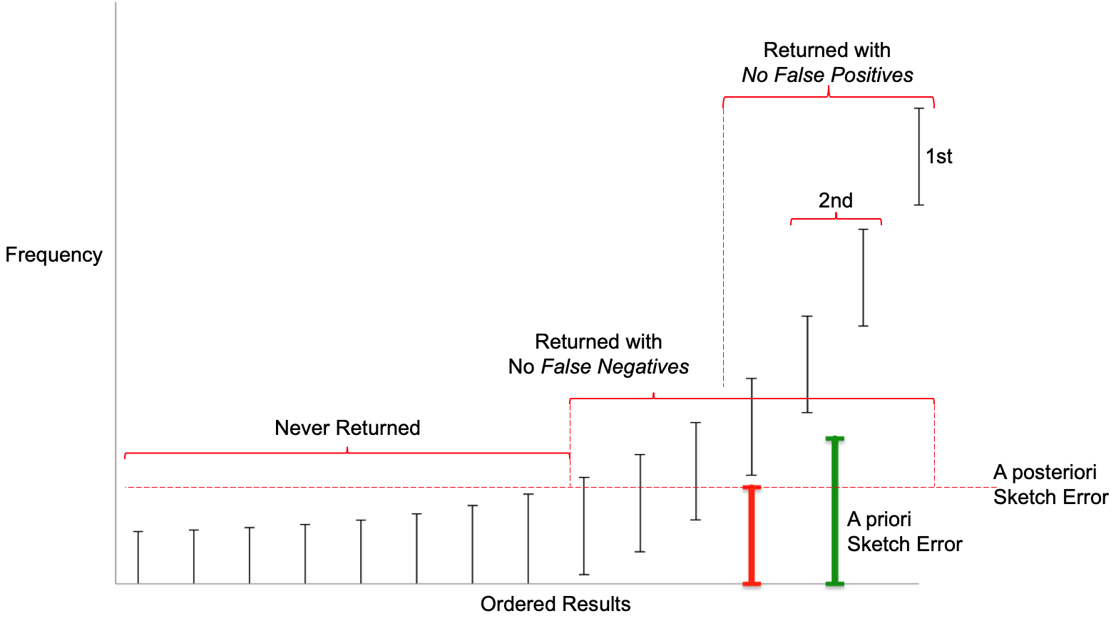
The above figure was created with synthetic data in order to illustrate a hypothetical set of returned results with their Error Bounds and how these Error Bounds interact with the two different Error Types chosen at query time. The black vertical lines with end-caps represent the items with their frequencies retained by the sketch. The upper end-caps represents the upper bound frequencies of each item and the lower end-caps represent the lower bound frequencies of each item. The sketch estimate for each item will be between those values inclusively.
The green vertical bar on the right represents the error computed from the above error table. It is an a priori error (or pre-error) in that it is computed before any data has been presented to the sketch.
The red vertical bar just to its left represents the a posteriori error (or post-error) returned by the sketch after all the data has been presented to the sketch and is often less than the pre-error. Note that the post-error is the same size as the error bounds on all the retained items in the sketch.
The post-error is used as a threshold by the sketch in determining which items, out of all the retained items, can be legitimately returned by the sketch.
In terms of order, only the first item on the far right can be safely be classified as the “most frequent” of all Items presented to the sketch. Because the upper and lower bounds of the next two items overlap, the next two to the left tie for second place. The next three to the left of those would tie for forth place, and so on.
These results can also be described using the classical “Confusion Matrix” as shown in the next figure.
Figure: Error Type and Confusion Matrix
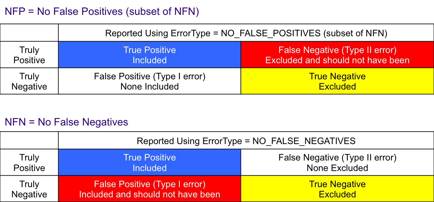
The items returned are represented by the blue “True Positive” box. However, there is the possibility that items, whose true frequency was above the post-error, might be excluded. These are the “False Negatives” represented by the red box and is classified as a “Type II Error”. No False Positives (Type I Error) are included. All True Negatives are excluded and there is no Type II Error.
For this Error Type, all the times returned by “No False Positives” are returned in addition to items classified as “False Positives”, or Type I Error. All “True Negatives” are properly excluded.
This code implements a variant of what is commonly known as the “Misra-Gries algorithm”. Variants of it were discovered and rediscovered and redesigned several times over the years:
We ran two sets of experiments, the fist generated a stream from a Zipfian distribution with alpha=1.1 (high skew), and the second with a Zipfian distribution with alpha=0.7 (lower skew). The frequency of an item i is proportional to 1/ialpha.
Figure: Real Count Distribution 1.1
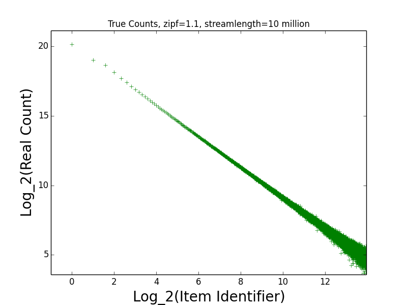 This is the empirical log-log distribution of the 10M random points generated.
Figure: Estimate Error 1.1
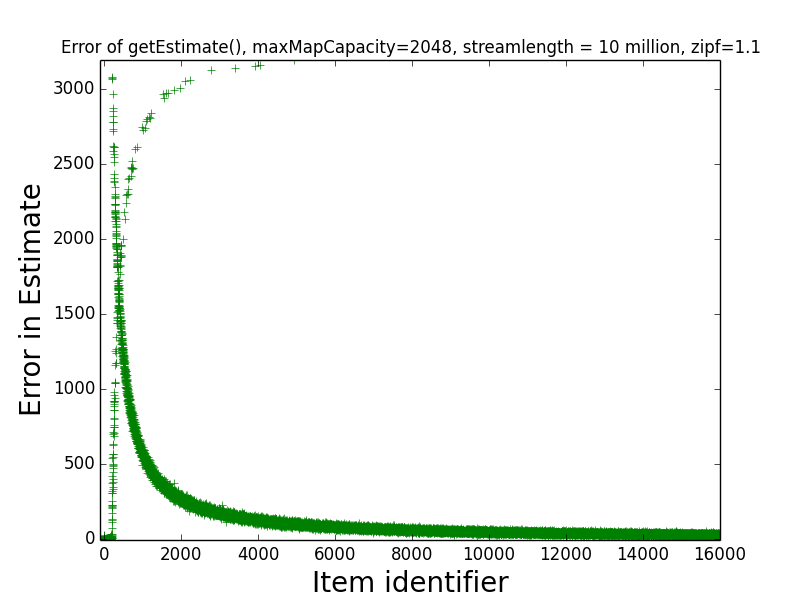 This depicts the absolute value of the error of the estimate
returned by getEstimate(item) for all items between 1 and 16000.
Several properties are worth noting.
This depicts the absolute value of the error of the estimate
returned by getEstimate(item) for all items between 1 and 16000.
Several properties are worth noting.
First, note the clustering of errors in the bottom left corner of the graph – this indicates that the estimates of the frequencies of most of the most frequent few hundred items are very close to exact (in fact, the maximum error for any of the first 189 items is just 7).
Second, note that, visually, two separate curves can be distinguished in the image, with one starting from the lower left corner and increasing toward the top right corner, and one starting from the top left corner and decreasing toward the bottom right corner. The first curve corresponds to items that were assigned counters by the sketch at the end of the data stream. The estimates returned for these items are always overestimates of their true frequencies, and these estimates tend to be more accurate for more-frequent items.
The second curve corresponds to items that were not assigned counters by the sketch when the last stream update was processed. For these items, getEstimate(item) returns an estimate of 0. Hence, the error in these estimates is exactly the true frequency of the items, which explains why the second curve starts in the top-left corner, and heads toward the bottom right.
Observe that the maximum error in the estimate of any item was slightly more than 3,000. This is much better than the “worst case error guarantee” for the sketch, which is W(3.5)(1/maxMapSize) = (10 million)(3.5)(1/2048) = 17,090. This indicates that on realistic data sets, the sketch is significantly more accurate than the worst case error guarantee suggests.
Figure: Get Frequent Items 1.1
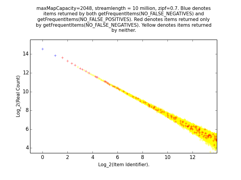
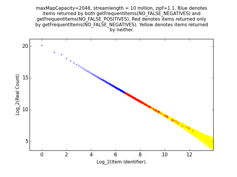 This is the log-log distribution of random points generated, color coded by whether
the points were returned by:
This is the log-log distribution of random points generated, color coded by whether
the points were returned by:
Recall that these functions return information about all items whose estimated frequencies are above the maximum error of the sketch, subject to the constraint that either all items whose frequency might be above the threshold are included (NO_FALSE_NEGATIVES), or only items whose frequency is definitely above the threshold are included (NO_FALSE_POSITIVES).
As expected, the most frequent items are returned by both function calls, while infrequent items are returned by neither. Items in between may be returned by neither, or by getFrequentItems(NO_FALSE_NEGATIVES) only.
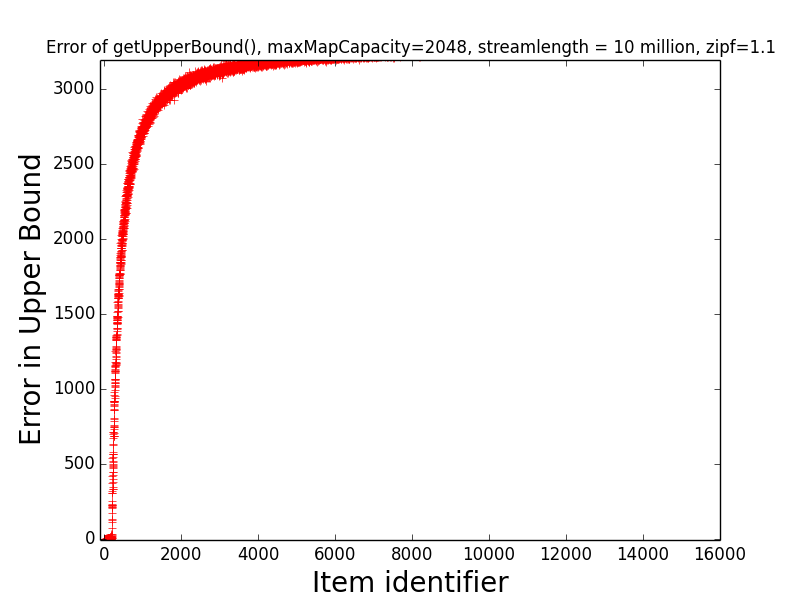
Figures: LB Error 1.1 and UB Error 1.1
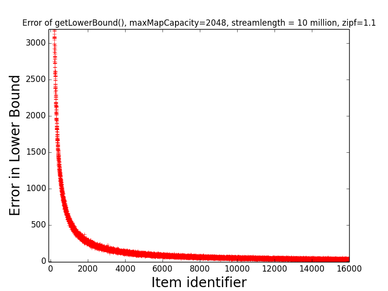
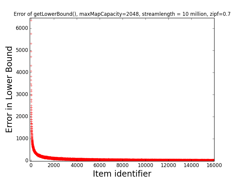
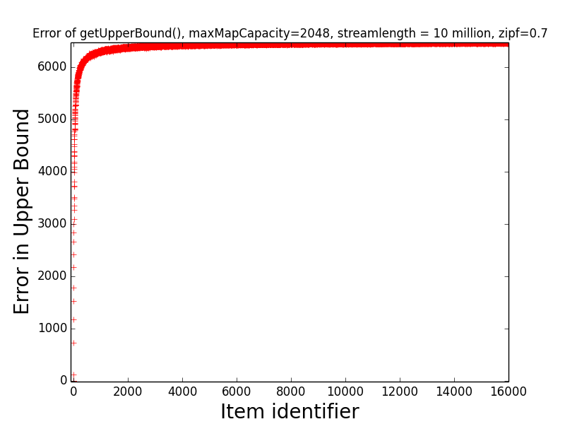
 The first figure depicts the error of get getLowerBound(item) for items 1, 2, …, 16000,
while the second figure depicts the error of getUpperBound(item) for the same items.
The first figure depicts the error of get getLowerBound(item) for items 1, 2, …, 16000,
while the second figure depicts the error of getUpperBound(item) for the same items.
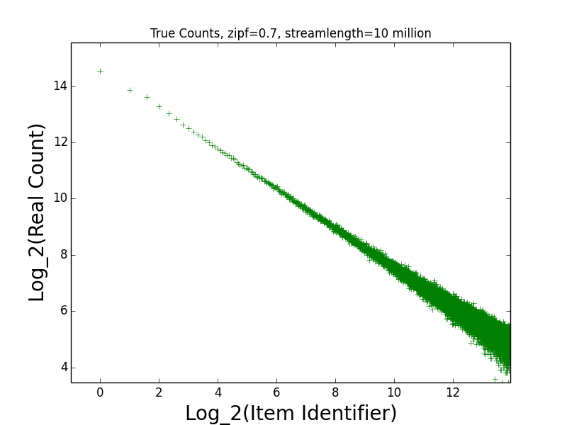
Figures: Real Count Distribution 0.7, Estimate Error 0.7, Get Frequent Items 0.7, LB Error 0.7 and UB Error 0.7
The following are the corresponding plots for a stream generated from a Zipfian distribution with parameter alpha=0.7.
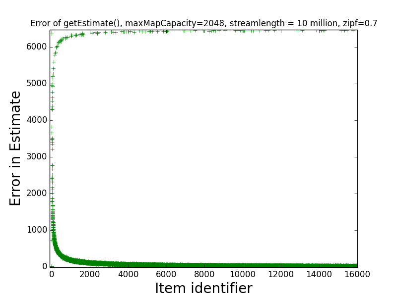
The main takeaway from these plots relative to the above is that the error in the estimates tend be higher than in the case alpha=1.1. Indeed, the maximum error in any estimate is nearly twice as large in the case alpha=0.7 than in the case alpha=1.1. Moreover, when alpha-0.7 only the estimates of the 6 most frequent items have error at most 10 when alpha=0.7, while in the case alpha=1.1, the estimates of all of the 189 most frequent items all have error at most 10. This higher error is also manifested in the fact that getFrequentItems(NO_FALSE_POSITIVES) only returned two items in the case alpha=0.7 (i.e., the two most frequent items in the stream), while getFrequentItems(NO_FALSE_POSITIVES) returned 101 items in the case alpha=1.1.
The reason for the increased error when alpha=0.7, is that the frequency distribution is flatter in this case. It well-known that the algorithms we have implemented perform better on streams where the most frequent items make up a larger percentage of the stream, essentially because the sketch is able to process these items with minimal or no error. See, for example, “Space-optimal Heavy Hitters with Strong Error Bounds” by Berinde et al. for formalizations of this property.
Finally, observe that the maximum error in the estimate of any item was slightly more than 6,000. This is much better than the “worst case error guarantee” for the sketch, which is W(3.5)(1/maxMapSize) = (10 million)(3.5)(1/2048) = 17,090. This indicates that on realistic data sets, the sketch is significantly more accurate than the worst case error guarantee suggests.
1 For speed we do employ some randomization that introduces a small probability that our
proof of the worst-case bound might not apply to a given run. However, we have ensured that
this probability is extremely small. For example, if the stream causes one table purge (rebuild),
our proof of the worst case bound applies with probability at least 1 - 1E-14.
If the stream causes 1E9 purges, our proof applies with probability at least 1 - 1E-5.

